

Introduction
A dataset arrives from somewhere else and the file listing tells you how many images there are and nothing else. Everything that decides what to do next - train on this, label more of it, throw it away - is in the annotations, and there is no way to read those by eye. Profiling the dataset gets you a report instead. This article is about reading that report: what each chart is for, what to look for in it, and when a shape on screen means something is wrong.
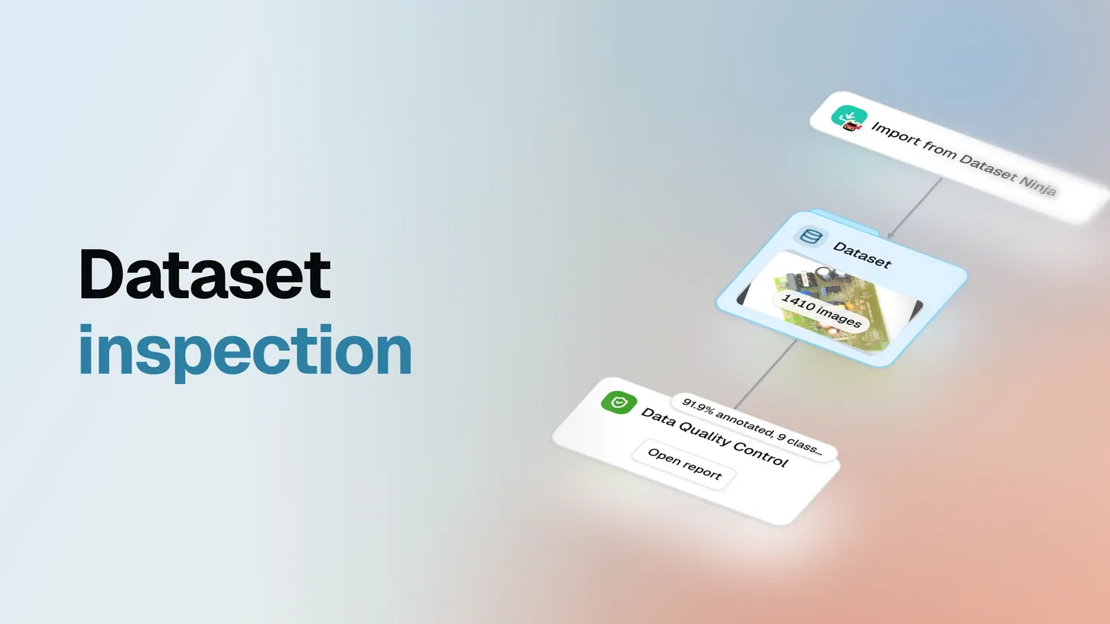
The example is PCB Component Detection - 1410 photographs of printed circuit boards, pulled from a public catalog and profiled in one step. It comes in three splits: 1099 images to train on, 200 to validate against, 111 held back as a test set, and that test split carries no annotations at all, which is normal and matters twice below.
Nothing about the dataset is special, and that is the point. Profile your own and you will get the same sections with different numbers, so read the charts for the method and the issues as an illustration of it.
The order to read it in
A report this size rewards being read in a fixed order, because each answer changes what the next number means. Seven questions, in this sequence:
- Is it all actually labelled? Coverage and issues, before anything else.
- Do the class names make sense? Read the list itself, not a chart.
- What will a model barely see? Class balance.
- How varied are the scenes? Class co-occurrence.
- How much is in one image? Objects per image.
- What is too small to learn? Object sizes, and their extremes.
- Does position give the answer away? Spatial distribution.
The report answers them in that order, one tab per section, and everything below walks the same route.
One habit to carry through all seven steps: in the report, nothing is a dead end. Every bar, slice and heatmap cell is clickable and opens the images behind it, and every table row opens that image with its annotations drawn on. A number that looks wrong is always two clicks from the pixels that produced it.
Every chart below is a live copy of this report’s data - hover them, read the exact values. What the copies cannot do is the clicking through: that path from a number to the images belongs to the report itself, and the Issues section shows what it looks like.
Coverage
Start with the least glamorous question. Not what is in the data - whether it is there at all.
The test behind that pie is stricter than most datasets apply to themselves: an image counts as annotated only when it carries at least one object, so a record that exists and holds nothing does not count. Which is why the number is 91.9% and not 100. Of 1410 images, 1296 carry objects and 114 do not.
Now the part that decides whether 114 is a problem: 111 of them are that test split, where having no labels is the point. The next section says so outright instead of leaving you to guess, and it matters because the two readings lead opposite ways - unfinished labelling is work to do, a held-out split is work already done correctly. Set those 111 aside and three images are genuinely missing their labels.
Worth keeping as a habit: a coverage number on its own is ambiguous by construction. Until you know which split an image belongs to, you cannot tell a defect from a design decision. The next pie is where that information lives.
Tags are how a dataset says what the pixels cannot: which split an image belongs to, which batch it
arrived in, which camera took it. Here there is one family of them - split: train on 1099 images,
split: validation on 200, split: test on 111 - and it pays to be precise about what that means.
The catalog declares those splits; this pie counts what actually arrived, and the two agreeing is
the check. A train slice reading 1097 would be the interesting case.
Two habits about the chart itself. An image is counted once per tag it carries, so a dataset tagged
along two dimensions - split and camera, say - produces slices that add up to more than the image
count; these sum to 1410 exactly because every image here carries one tag. And images carrying no tag
get a slice of their own, which is the shape worth recognising: a small tagged slice beside a large
Untagged one is how a tag applied to a handful of images by accident announces itself.
The third pie changes subject, from images to the objects inside them.
Read this one for proportion and nothing else - exact per-class counts arrive two sections down. What
you want to notice is any segment large enough to dominate a loss function. Transformer takes
roughly a quarter of all objects, which is a mild imbalance and no cause for alarm. The part worth a
second look is Other: two classes small enough that the chart would rather not draw them.
Issues
Coverage counted the images. This section names the problems, and it comes second in the report for a reason: everything below is easier to read once you know what the data is already accused of.
The tile gives a count of four; the tab gives one row per issue, with the images behind each one a click away. The whole table fits here:
| Issue | Severity | Images |
|---|---|---|
| Images with no labels | Check | 3 |
| ‘Resestor’ may be a misspelling of ‘Resistor’ | Check | 3 |
| ‘Resestor’ is rare: 0.21% of the images | Check | 3 |
| ‘Resestor’ is labeled only in val | Check | 3 |
Read the last three rows together. They accuse the same class from three directions - the name looks
like a typo of Resistor, the class covers 0.21% of the images, and every image it touches sits in
the validation split. Three independent checks converging on one class is about as loud as a
statistics report gets, and the proof arrives two sections down.
The first row is a different problem. Its three images turn out to be one video frame exported three
times under different .rf.<hash> names - click the row and the previews show the same board thrice.
Worth knowing before you plan the fix: this is one photograph to label, not three.
Notice also what is not in the table. The other 111 images without objects are the test split,
expected to arrive unannotated - the report says so in a sentence over the table instead of flagging
them, and that restraint is doing real work: a profile that cried about all 114 would have sent you
hunting 114 problems, of which three exist. And the two twenty-pixel MOSFET boxes you will meet in
the size sections are not here either: issues cover bookkeeping and suspicious names, while
judgements about sizes stay in the charts, where the thresholds are yours to set.
Clicking a row answers the question a count cannot: what is actually wrong with this board?
The board is fine. The annotation work is not - and no aggregate could have told you which of those two it was.
That route is open from every chart in the rest of the report, not just this table: a bar, a pie slice or a heatmap cell is a filter over the dataset, and clicking it puts the images behind the number on screen. It is the difference between reading a report and auditing a dataset, and the sections below are worth reading with a mouse rather than only with your eyes.
Class names
Before any chart, read the class names themselves. It takes ten seconds:
Cap1, Cap2, Cap3, Cap4, MOSFET, Mov, Resestor, Resistor, TransformerFour capacitor grades, a MOSFET, a varistor (Mov), a transformer, Resistor - and Resestor,
which is Resistor misspelled. Two classes for one component. Nothing in the pipeline flagged it,
because nothing in the pipeline reads English: the name arrived from the source annotations and was
carried faithfully through the catalog and the import. Every chart from here on has nine categories
where it should have eight, and the ninth is about to teach us something.
Image resolutions
Some charts are informative because of what they plot. This one is informative because of its shape.
Each point is one image size, placed by width and height, and the bigger the point the more images share it. On a dataset with a native resolution you would see one heavy dot and little else. Here there is no heavy dot to find: 1410 images spread over 405 distinct sizes, and the most common size accounts for just 13 images.
That shape tells you two practical things: read object sizes as percentages of the frame rather than in pixels, and expect no shortcut when you set up training input. It also shows where the sizes live - the cloud has structure a ranked bar chart could never show, portrait and landscape groups sitting apart.
Class balance
Two bars per class: images containing it, and objects of it. The gap between the pair is where the information is - equal bars mean about one instance per image, a taller object bar means the class arrives in multiples.
Usually you open this chart to find a rare class drowning under a common one. Not here. Eight of the
nine classes sit on a plateau between 1062 and 1295 images - they are all common, all at once -
and only Transformer shows an object bar visibly double its image bar.
The ninth class is the sliver you cannot see at this scale.
| Class | Images | Objects | Avg object area |
|---|---|---|---|
| Transformer | 1295 | 2547 | 4.99% |
| Cap1 | 1295 | 1295 | 2.90% |
| MOSFET | 1293 | 1295 | 1.80% |
| Mov | 1291 | 1291 | 2.81% |
| Cap2 | 1264 | 1264 | 1.32% |
| Cap3 | 1199 | 1199 | 2.99% |
| Resistor | 1145 | 1151 | 0.80% |
| Cap4 | 1062 | 1074 | 2.99% |
| Resestor | 3 | 3 | 1.03% |
Three objects, against 1151 for the correctly spelled class. When something sits three orders of magnitude below its neighbours, stop asking whether a model can learn it and start asking whether it should exist.
Class co-occurrence
This is the chart that changes how you read all the others.
Each cell counts the images holding both classes; the diagonal counts images holding that class at all. A healthy matrix has structure - dark clusters where classes travel together, gaps where they never meet. This one is almost uniformly saturated. Every pair of the eight real classes shares at least 986 of the 1410 images, and most pairs more than 1200.
That is not a varied collection of boards. It is one board layout, photographed over and over.
The same heatmap also settles the typo, in the one cell that stayed white. Resestor shares images
with every other class exactly three times - and with Resistor zero times. In a dataset where
Resistor appears in 1145 of 1410 images, the three images holding the misspelled class are
precisely the three where the correct one is missing. That is not a rare component. That is a name
typed wrong three times.
The Issues section above reached the same conclusion from the other direction, by comparing the
names themselves: 'Resestor' may be a misspelling of 'Resistor'. But a flag is a suspicion, and
this cell is the proof. Clicking it opens the three images behind it, so the whole check takes about
two seconds.
Objects per image
Labelling density is usually a gentle hump. This one is a cliff.
979 of the 1410 images carry exactly nine objects. Another 168 carry eight. Below seven there are only handfuls - 3 images with three objects, 1 with four, 18 with five, 31 with six - and then a gap where nothing lives at all: no image carries one or two objects, while 114 carry none.
The gap says the work was all-or-nothing: a board was labelled completely or not at all, never half-way. The bar at zero is the 114 from the coverage pie - mostly the test split, three of them actually missing - so read it as two different things stacked in one bar, which is exactly why the Issues section separates them for you.
Nine is a suspiciously specific number, and the per-class view explains it.
Seven classes never contribute more than one object to an image. Transformer contributes two in
1252 of them. Seven singles plus two transformers is nine - the modal board, repeated 979 times.
The only deviations in the entire dataset are Cap4 twice in 12 images, Resistor twice in 6, and
MOSFET twice in 2. Any of those cells is clickable, so the twelve Cap4 doubles are one click away
if you want to know whether they are real or a labelling slip. The Resestor row, meanwhile, is the
clearest possible portrait of a ghost class: 1407 images with none of it, three with one.
Put that beside the saturated co-occurrence matrix and the conclusion is hard to dodge: the same board, over and over. The report cannot tell you that - it counts labels, it does not recognise hardware - but a fixed object count built from a fixed class recipe is what a single repeated subject looks like in statistics.
Which matters before you split the data. A random train/test split over 1410 photographs of one board hands you a test set that is another photograph of something the model has already seen.
Object sizes
Averages tell you which classes are small. The ends of the whiskers tell you which annotations are broken.
On averages alone the spread is a factor of six: a transformer covers 4.99% of the frame, a
resistor 0.80%. Worth noticing along the way that Cap2 at 1.32% is less than half of Cap3 and
Cap4 at 2.99% - grades that share a prefix are not the same size of thing.
The extremes are where the chart earns its place. Transformer runs from 0.54% to 15.83%, a
factor of twenty-nine inside one class, which is what a moving camera does to relative area. And at
the very bottom sits a genuine defect: the smallest MOSFET box covers 0.0011% of its image. On a
1860 by 1046 photograph that is about twenty pixels of area - a box nobody drew deliberately and no
model can learn from.
Small classes stay hard, for what it is worth: in the two published studies that trained detectors on
this data, the weakest real classes were Resistor and Cap2 - the two smallest here.
Size distribution
The same measurement, spread across ten buckets. Read this one from the edges inward, because the edges are where mistakes collect: anything under 0.05% of the frame is almost certainly broken, and anything over half the frame is a box that swallowed the image.
Both edges come back nearly clean. The mass sits where it should, in the 1-2% and 2-5% buckets, and the only occupants of the extremes are two MOSFET objects under 0.05% - the twenty-pixel box and one sibling. Two broken boxes out of 11119 is a good dataset by any standard; the point is that you now know the number instead of assuming it, and clicking that leftmost bar puts both of them on screen.
The colours double as a size ranking, incidentally: Resistor sits almost entirely in the 0.1-1%
band, Transformer in 2-10%.
Spatial distribution
Every image is divided into the same 16 by 16 grid, and each cell counts the bounding-box centres that land in it - row 1, column 1 being the top-left of the frame. An even spread means position tells a model nothing. A hot spot means position tells it everything, and a model that learns location instead of appearance scores well in testing and fails in production.
The report draws one map for all classes together and one for each of the three largest. They answer different questions. The combined map is about the photography.
Every side has an empty margin: the boards are centred in frame and nothing is ever labelled at the edges. That is a property of the shoot rather than of the data - a model trained here never sees a component near a frame edge, which is worth knowing if production images are cropped differently.
A single-class map is about the board.
Here the layout leaks through. Transformer puts 46% of its objects into its top 16 cells, and
Cap1 - the next map in the report - touches only 125 of the 256 cells, with half of its 1295
objects in 16 of them. Each component keeps to one region because it keeps to one place on the
board.
Note what this is not, though. A fixed camera rig would give you a few blazing cells and nothing else; instead the heat spreads over roughly a quarter of the frame, and the all-classes map touches 238 of 256 cells. The framing moves from shot to shot even though the subject does not - a more useful conclusion than either extreme, and it took one glance. Hot cells are clickable as well, which is the quickest way to check whether a bright spot is a real pattern on the board or a handful of mislabelled boxes piled in one corner.
Geometry
One slice: all 11119 objects are rectangles. That full circle is the good outcome, and it takes thirty seconds to confirm.
Here is why it is worth those thirty seconds. Width, height and position in this report come from an object’s enclosing rectangle, not from its labelled pixels. On a dataset mixing boxes with masks and polygons, the size statistics above would mean different things for different classes, and the comparison you just made would be quietly wrong.
What one pass found
None of the above set out to audit this dataset. The seven questions were asked in order, each chart read for what it is for, and these are the things that fell out on the way - from an ordinary public dataset that nobody had flagged as broken:
- A class that should not exist.
Resestor, 3 objects against 1151 for the correctly spelledResistor. The report accuses it three ways - a suspected misspelling, rare at 0.21% of the images, labeled only in the validation split - and the zero cell in the co-occurrence matrix turns the suspicion into proof. - Two boxes no model can learn from. Degenerate
MOSFETlabels around 0.0011% of their images, roughly twenty pixels of area each, alone in the leftmost bucket of the area histogram - a chart-level catch, not an issues row. - Three images that really are missing labels - as opposed to the 111 that are simply the test split. Telling those apart is the difference between three fixes and 114 imaginary ones.
- A test set that is not independent in the way that matters. Saturated co-occurrence, a fixed object count and concentrated spatial maps all say the same thing: one board layout, photographed 1410 times. The split is honest; the diversity behind it is not.
Three of those are small, concrete fixes. The fourth is not fixable at all - it is a fact about the data you have to design around. That is a fair return on a step that trains nothing and takes one run, and your dataset will produce a different list from the same seven questions.
Limits
Three things the report does not do, so you know where it stops:
- Judge a label. It compares class names, which is how
Resestorsurfaces, but never looks inside a box. - Say anything about a model. No accuracy, no readiness to ship.
- Change the data. Everything above is an issue; the dataset is exactly as it was.
Acting on issues like these - repairing what the table names, and proving the repair with a second profile - is the next study, and it picks up this exact report where this article leaves it.
Takeaway
A profile is the cheapest step in the pipeline: no labelling, no training, one run. What it buys is a set of answers that otherwise arrive late or not at all - which classes a model will barely see, how alike the images really are, which annotations are broken, and which of the odd-looking ones are actually fine.
That last part is the underrated half. A count of images without labels means nothing until you know which of them were supposed to have none, and a report that keeps the two apart saves you from fixing things that were never broken.